We used Kalman filters and residuals to determine whether there was a problem with the REPOINT mechatronic switch for railways. After prototyping this in simulation, we found that it worked. Then, we applied this to a scale model of a mechatronic switch to check if it worked there too. And it did!
Motivation
Most railway switches (or points) are purely mechanical and use super-old technology to switch between tracks. This would be fine, except that they are the #1 cause of delay minutes on the UK rail network! The REPOINT project aimed to reduce these failures by replacing these with mechatronic switches that had in-built sensors and which were easily lineside replaceable.
But, it wasn’t clear how these mechatronic switches would deal with a sensor failure. Or how it might recover from one.
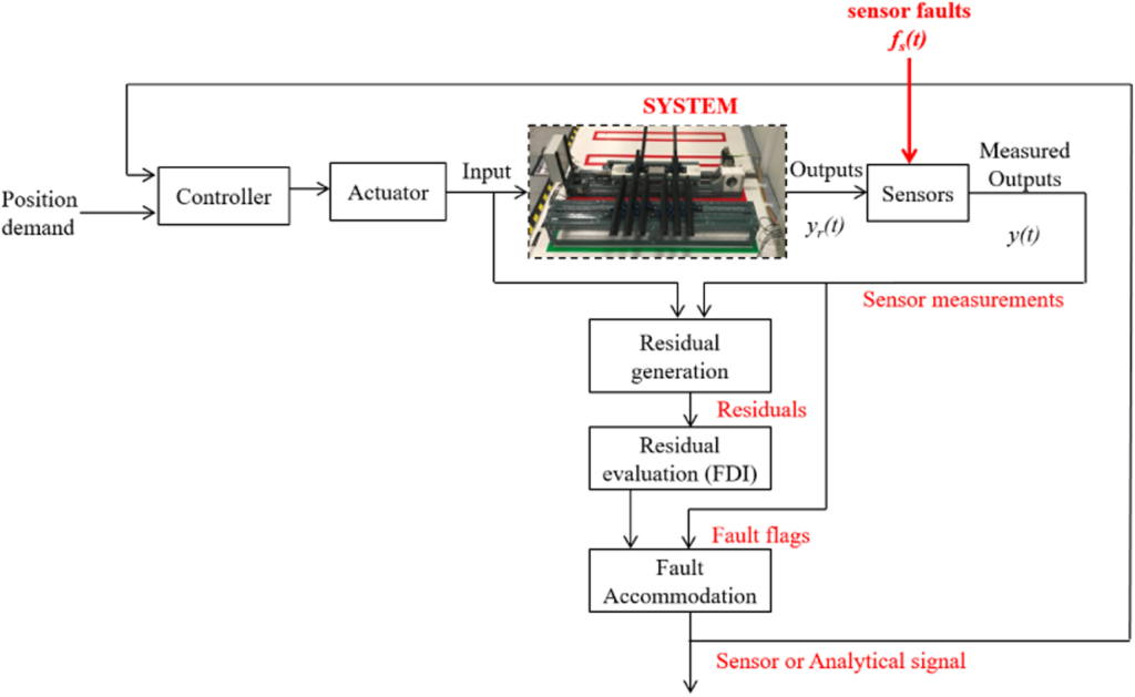
An overview of the mechatronic switch, showing where the faults could occur.
Mechatronic Switch Simulation
We focussed on disconnect failures, where one of the signals (either position or velocity) was disconnected from the controller. To see what effect this would have, we first built a software simulation of the mechatronic switch.
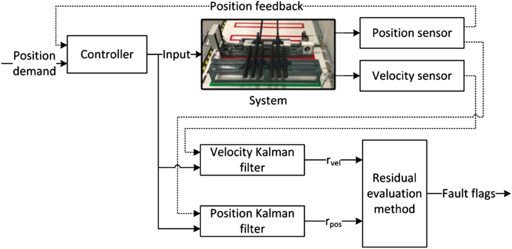
An overview of the fault detection system for the mechatronic switch
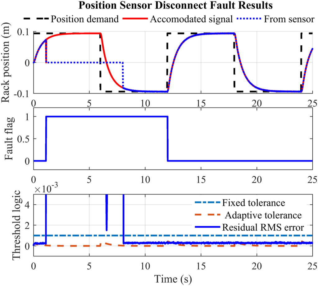
Then, we used the Kalman filters to estimate what the states of the system should have been. In the figure below, you can see that the signal from the sensor (in blue dashes) drops to zero, but the filter’s estimate of the signal (in red) tracks correctly. That’s pretty cool!
Showing how the Kalman filter estimate (red in top axes) continues to track the motion of the system even when the position sensor (blue dashes in top axes) is turned off.
The Real Deal (AKA: The Real Mechatronic Switch)
Then, we took this scheme and applied it to our small-scale model of the REPOINT switch:
Overview of the small-scale model of the REPOINT switch
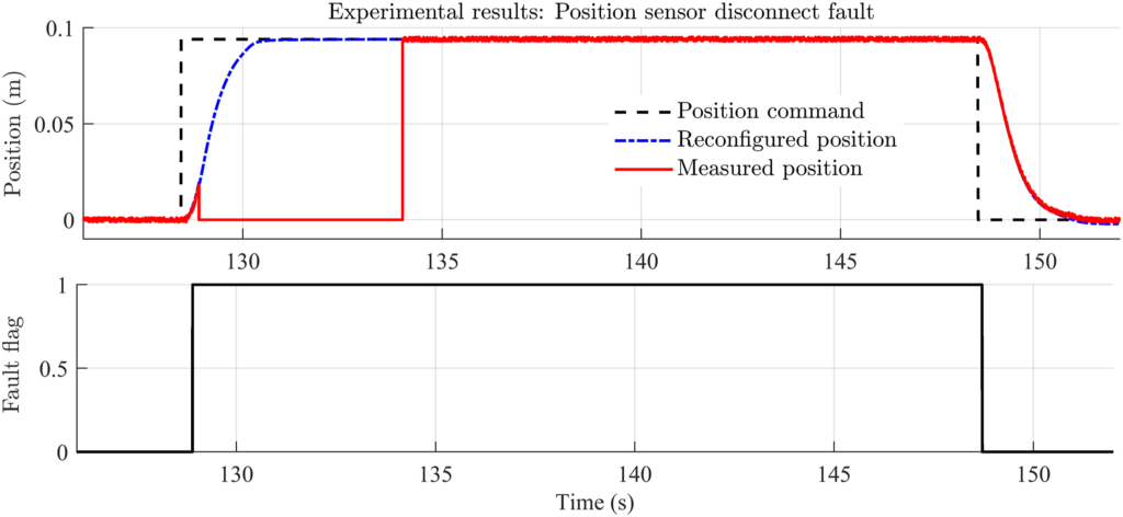
Long story short – it worked! When we used some logic to determine when to trust the Kalman filters over the sensor signals, the system was able to continue to work when the position or velocity sensors were disconnected. (This approach uses thresholding of the residuals – more information is available in the paper.)
Showing the response of the physical model, and the ability of the Kalman filters to correctly estimate the mechatronic switch’s position.
Conclusions
It worked! Using Kalman filters and residual logic, we were able to ensure the switch could continue working even if one of the sensors failed. Pretty neat eh!
Acknowledgements to Dr Precious Kaijuka Mwongera who did the experimental work for this paper!
We looked at several different control algorithms that might be used to reduce torque ripple (unwanted wobbles in the output of electric motors). We built a mathematical model of the controllers and ran them to see how they performed. (As well as checking them mathematically.)
Our analysis showed that a lot of these torque ripple control algorithms were mathematically very similar. They also behaved very similarly in simulations. The best algorithm we found was called PIR-A. This controller was a resonant proportional-integral controller with added phase advance.
Motivation
Torque ripple is an unwanted side-effect of the way we build permanent-magnet synchronous machines (PMSMs). It makes them less efficient and less controllable. We wanted to look at how different torque ripple control algorithms worked on a simple simulation.
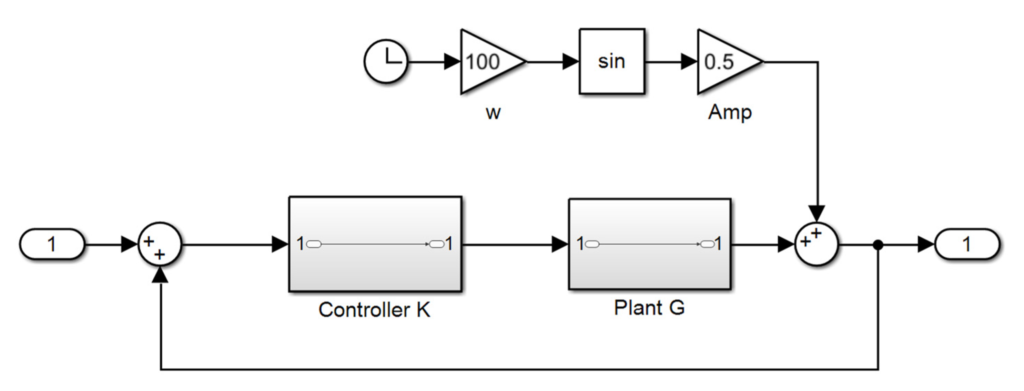
Overview of simple simulation
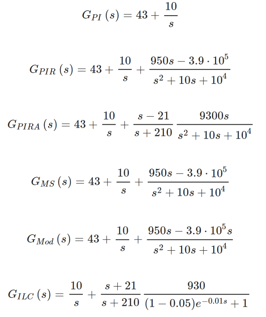
Controller Summary
Torque ripple is a cyclical phenomenon (due to the radial symmetry in the machine), meaning some traditional controllers don’t reduce torque ripple. With this in mind, we looked at 6 controller variants:
Proportional-integral control (PI). This is a standard controller, not well suited to dealing with cyclical phenomena.
Proportional-integral resonant control (PIR). A resonator is added to a normal PI controller to try and address the cyclical disturbance.
Proportional-integral resonant with phase advance (PIRA). This adds phase advance to the PIR control to try and reduce the effects of the introduction of the resonant bit.
Mixed sensitivity design (MS). We used optimal control approaches to design a controller to reduce disturbances around the torque ripple frequency.
Modulating controller (Mod). We applied modulating control theory to design a controller to reject disturbances specifically at the torque ripple frequency.
Iterative learning control (ILC). This controller tries to learn the disturbance from previous cycles to determine the best remedial action for the following cycle.
Next, when we compared the different approaches, we found that they all looked pretty similar! (Apart from the PI – it doesn’t have any specific additions to deal with cyclical disturbances.)
Bode Plots (Frequency Response)
When we looked at their behaviour, we saw that they looked pretty similar too:
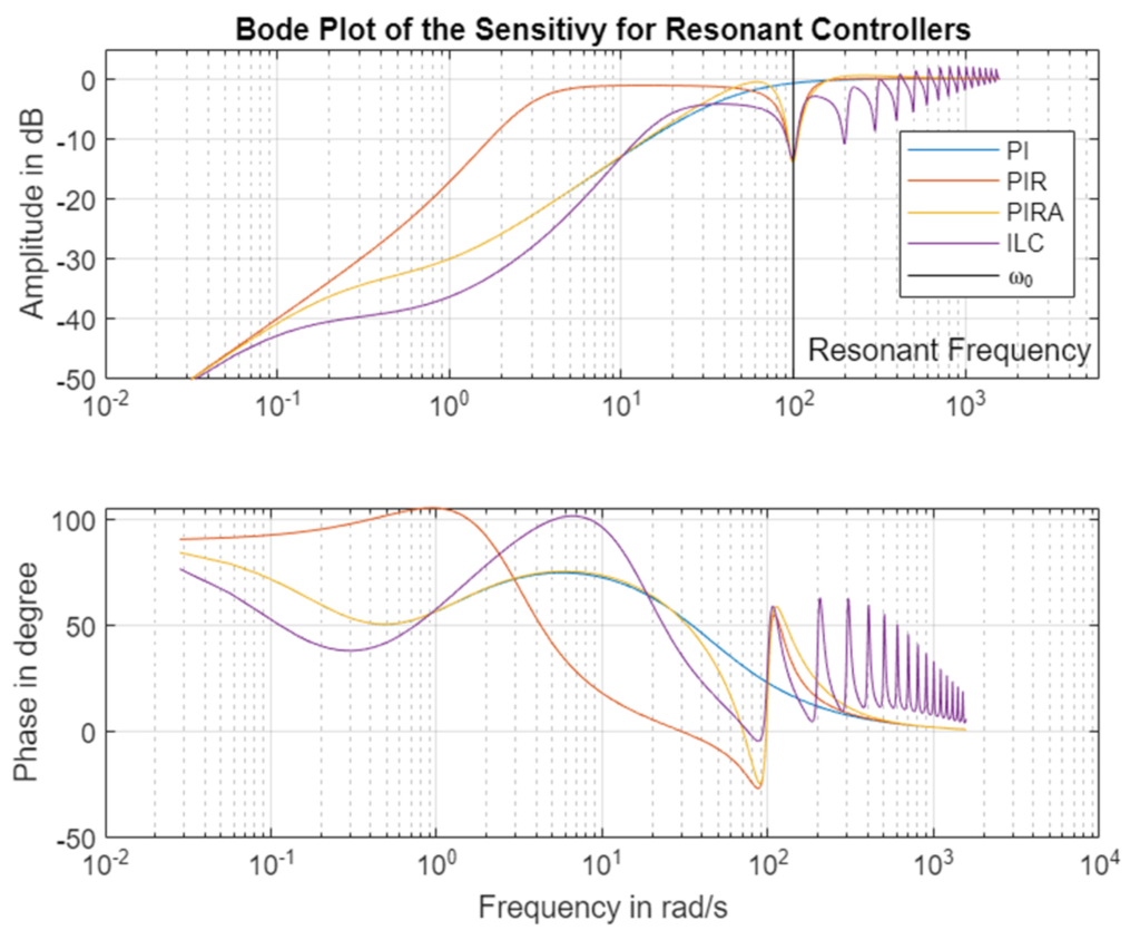
Closed-loop Bode plot of the different torque ripple control algorithms
In the figure above, you can see the dip in gain around the disturbance frequency, ω0, which is good – it means the disturbance is being filtered out by the controller. (Apart from PI, which doesn’t make allowances for the resonant disturbance.)
What is interesting here is that the PIRA controller that we designed has very similar low-frequency behaviour to the PI controller. That means that it’s behaviour in this region is pretty good, plus it has the dip at ω0! Also interesting here is the behaviour of the ILC. It has a ‘comb-like’ behaviour after ω0, which corresponds to higher harmonics of ω0. This might be good, if we know the disturbance is also at higher harmonics, but it might also make things difficult if we have noise or other machine properties at these frequencies.
Time Domain Response
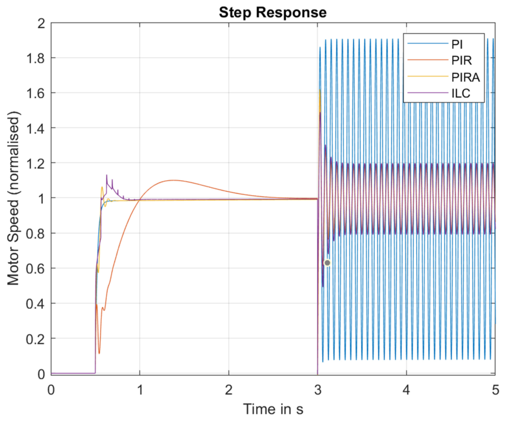
Then, we looked at the response of the different torque ripple control algorithms in the time domain. We looked at the step response of the closed-loop system, followed by its response to the introduction of a resonant disturbance:
Step and resonant response of the different control algorithms
Here we can see a few interesting things:
The PI controller has really good step response (it reacts quickly and has little overshoot), but performs very poorly when the resonant disturbance is introduced at t=3 seconds.
the PIR controller has slow step-response behaviour but does reduce the torque ripple.
The ILC controller has strange step response behaviour, which is likely due to the ‘comb-like’ bode plot interacting with the broad range of frequencies present in a step response.
The PIRA controller has good step response characteristics and also reduces torque ripple.
There is more work to do here. Specifically, we’d like to run the controllers on real hardware to see if our conclusions still hold. We’d also like to make the base control model a bit more complex, to see if our algebraic assumptions still work.
Conclusions
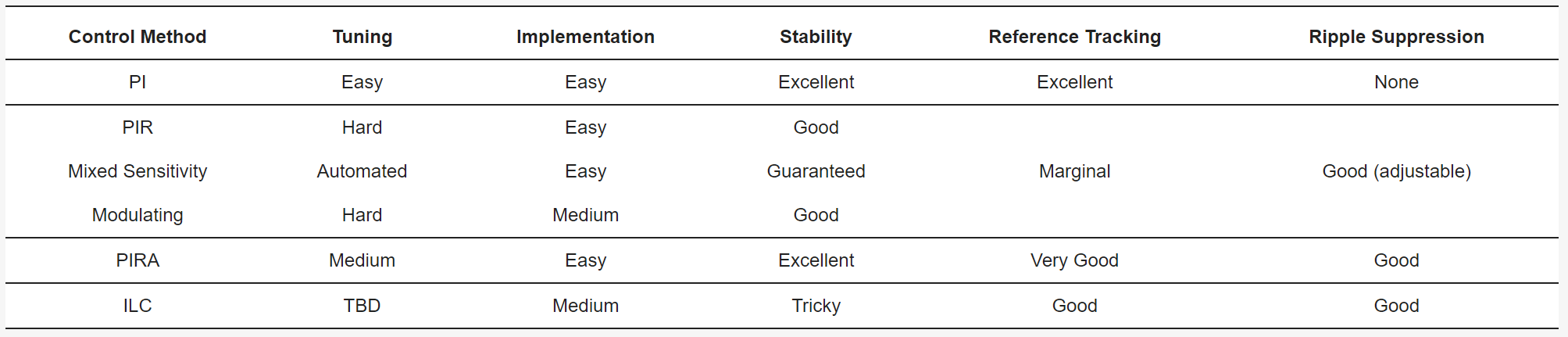
We boiled it all down into one handy table which shows how the different torque ripple control algorithms compare:
Table showing a comparison of the different control algorithms.
We applied systems-engineering techniques to investigate how municipal solid waste (MSW) is treated, using Saudi Arabia as a case study. We built a mathematical model of the system and used it to investigate different scenarios.
This model showed that a combination of anaerobic digestion (for food and organic waste), recycling and incineration (for non-recyclable materials) would reduce the total mass of waste to landfill by 73%. Not only that, this approach reduced the effect of the waste management on the environment by 98%.
Motivation
In Saudi Arabia, municipal solid waste (MSW) is currently disposed of in landfill (dumping it in a hole). This causes irreparable environmental harm and increased hazard from the possibility of landfill fires.
However, the Saudi MSW system is a large, multi-stakeholder (lots of people are interested in the outcome) system. This makes it a great system to develop “nation-scale” (really big) systems engineering tools on.
System Model
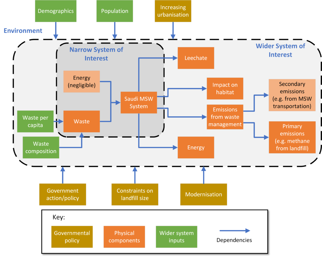
My previous work has focussed on modelling rail vehicles and infrastructure, and using these models to investigate how to reduce their emissions. So we took that and applied it to this giant system – the Saudi MSW system:
System overview showing how different factors (government policy, physical constraints and wider system inputs) effect the environmental effects of solid waste disposal.
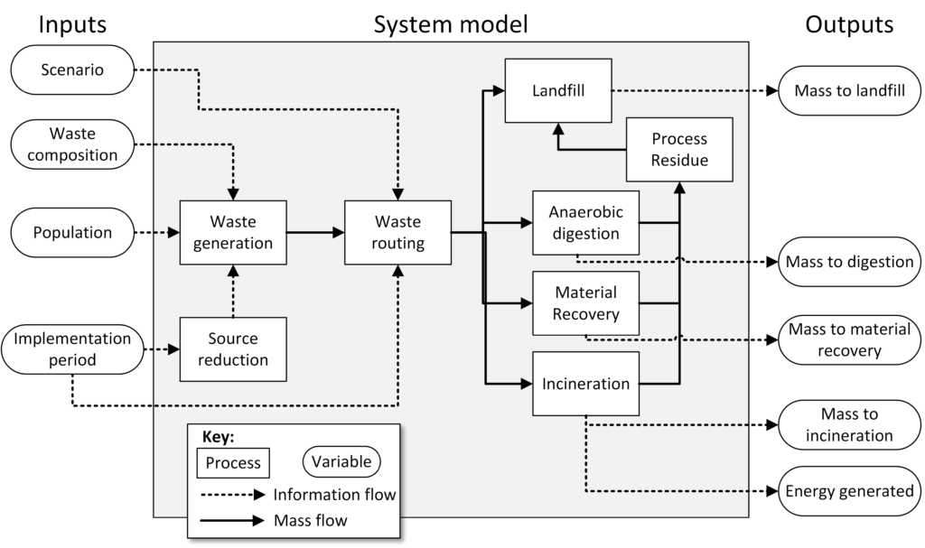
Then we built a mathematical model of the system, so that we could understand how the narrow system of interest (the waste stream) behaved when we changed some of the inputs. (This involved lots of checking through other people’s work to see how these things should be modelled!) Finally, we came up with a (pretty complex!) system model that looked like this:
Schematic of the detailed system model of Saudi Arabia’s municipal solid waste system.
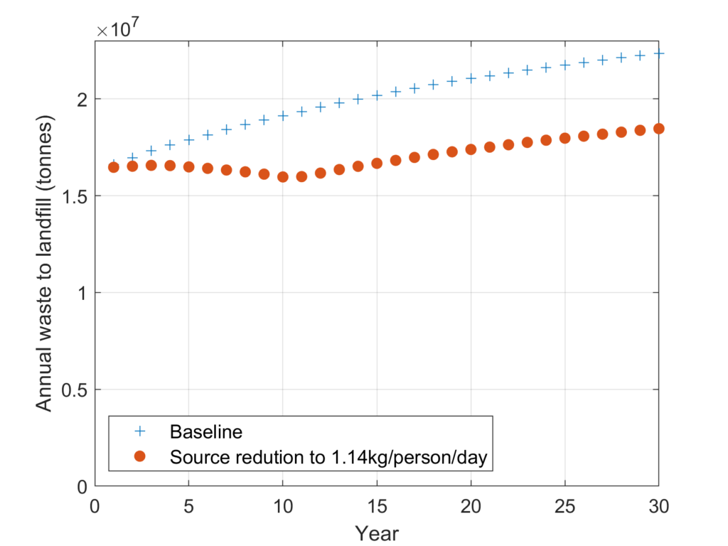
Then, we made some assumptions about about the makeup of the waste, and the likely population growth over the next 30 years. With that done, we could then answer two basic questions: What happens if we do nothing? What happens if Saudi citizens reduce their waste per person from 1.38kg/day to 1.14kg/day (in line with the UK)? And the answer is:
How much waste to landfill? ‘Baseline’ is if nothing is done. ‘Source reduction’ is if Saudi citizens reduce their municipal solid waste to 1.14kg/day, in line with the UK.
Using the Model
Then, we took this freshly made model and applied it to a range of possible scenarios that we’d devised, based on what we would do, and what other people had suggested:
Scenario number
What it involved
Scenario 0 (baseline)
Everything to landfill
Scenario 0.1
Everything to landfill, but less waste per person (1.14 kg/person/day)
Scenario 0.2
Everything to landfill with much less waste per person (1.02 kg/person/day)
Scenario 1
Food, glass and metal to landfill. Everything else is incinerated
Scenario 2
Everything except glass and metal goes to anaerobic digestion
Scenario 3
Anaerobic digestion or recycling for everything. (Incineration for textiles)
Scenario 4
Anaerobic digestion or recycling for everything. (Landfill for textiles)
A quick summary of the scenarios used in the study, showing where all of the waste ended up.
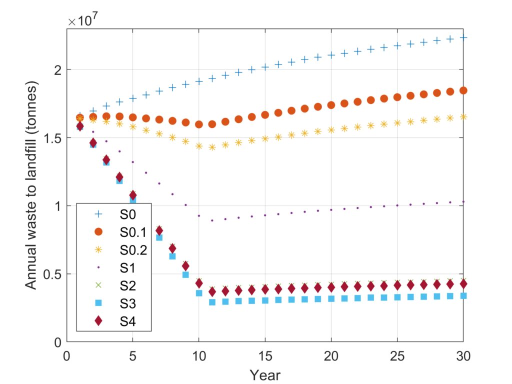
And this gave us some pretty graphs, showing how much waste went to landfill in each year for each of the scenarios. (Each of the measures was given 10 years to implement, because making new infrastructure takes time.)
Graph showing how much waste goes to landfill each year under each of the simulation scenarios.
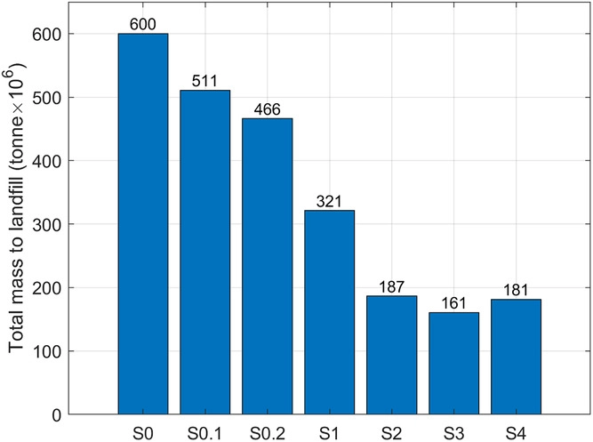
Then, we could look at how much went to landfill in total over the 30-year horizon of the simulation:
The total mass to landfill over the 30-year horizon for each of the scenarios.
This is pretty clear! S3 leads to the lowest total mass to landfill over the 30 years of the study. Job done!
Environmental Impact
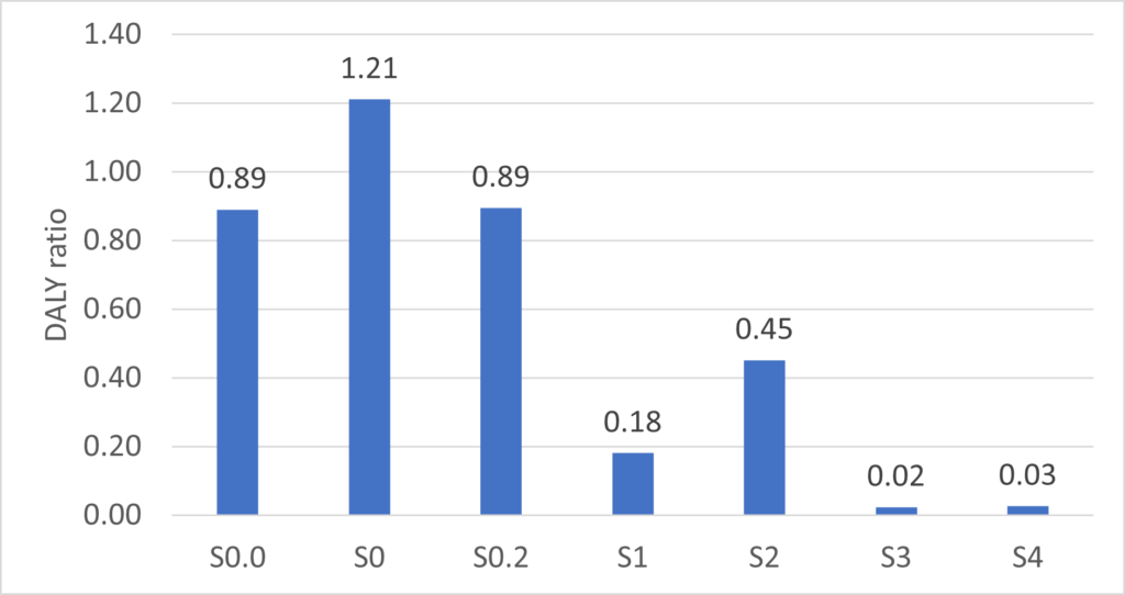
Well, almost. Finally, we wanted to check how the environmental effects of each of the scenarios compared. For this we used a commercial life cycle analysis (LCA) tool called SimaPro. We modelled each of the scenarios in this tool, and compared the DALY for each of them. (DALY stands for disability-adjusted life year, or how much of an effect a certain action has on people’s lives. The higher the number, the worse the effect on us.)
The relative DALY (disability-adjusted life year) for each different scenario. These have been normalised so that Scenario 0.1 = 1. For example, in this case Scenario 0 (not doing anything) is 28% worse than Scenario 0.1 (moderate reduction in waste per person per day).
You can see that all of the changes suggested by our systems engineering for waste management study have reduced the hazard the waste poses to people’s lives. In fact, Scenario 3 has only 2% of the impact on people’s lives of the current system. This is encouraging!
Conclusions
The results of this study into systems engineering for waste management are encouraging!
Just reducing the amount of waste people create would reduce the amount of waste to landfill by 89 million tonnes over 30 years.
Scenario 3 (anaerobic digestion of most waste, combined with recycling and limited incineration of non-recyclable materials) is the winner! This would save 328 million tonnes of waste going to landfill over the next 30 years.
Scenario 3 also reduces the impact of waste management on people’s health by 98% compared to the current system.
Other work
For more information on my research, please check out my Research page.
(Intermittent electrification means electrifying parts of a rail route, rather than the whole thing.)
Paper Overview (TL;DR)
We used a model of a train to investigate how intermittent electrification can help reduce carbon dioxide emissions in the near term. (The long-term goal should be to electrify everything!)
Using intermittent electrification can reduce carbon dioxide emissions by 54%, increasing to 59% if we include the CO2 embodied in the electrification infrastructure.
Motivation
Electrification is expensive, costing around £1.5 million – £2.5 million per single-track kilometre. It also takes a long time – these are large infrastructure projects that take time to deliver. Instead of continuously electrifying from (e.g.) London outward, intermittent electrification could reduce cost and provide decarbonisation faster.
As we already had a rail vehicle model from previous work, we used this to investigate!
The Rail Vehicle Model
The rail vehicle model was based on the model developed in earlier work. Next, it was extended to include the intermittent electrification to allow it to switch between overhead line equipment (OLE) and the on-board diesel engine.
Intermittent Electrification Model Results
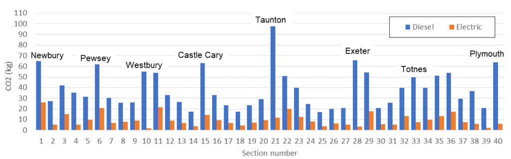
We ran the model over the route from London Paddington to Plymouth in both diesel and electric modes. Next, we compared the two, which showed us where CO2 emissions were the greatest along the route.
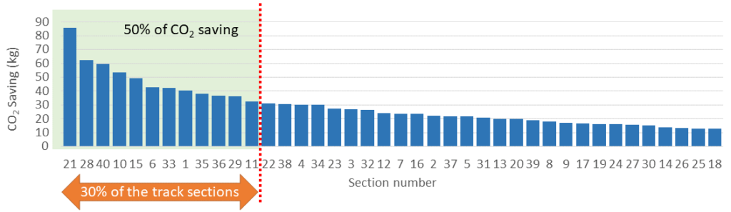
The carbon dioxide emissions from different sections of the route between London and Plymouth.
This allowed us to check how electrification would affect the carbon dioxide emissions of the route. We found that 50% of the carbon dioxide savings came from electrification of 30% of the track!
When the sections are ranked by carbon dioxide saving from electrification, 50% of the saving comes from electrifying 30% of the track.
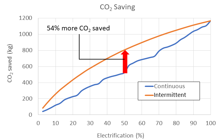
In fact, intermittent electrification produced higher carbon dioxide savings than continuous electrification across the board!
At 50% electrification, intermittent electrification saves 54% more CO2 than continuous electrification.
Whole-life Carbon Dioxide Emissions
Until this point, we had been looking at ‘operational’ carbon dioxide emissions. (These are emissions that come about from running the trains on the railway.)
However, electrifying track requires steel, concrete and machinery to string up the wires, all of which produce carbon dioxide. So, the next step of our analysis investigated the ‘whole-life’ emissions of the railway, including an estimate for the carbon dioxide emitted during electrification.
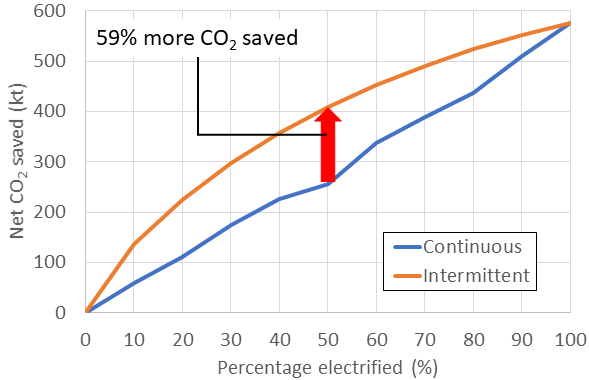
Including industry-recognised numbers for the carbon cost of electrification, we found that intermittent electrification saved up to 59% more carbon dioxide than continuous electrification.
Intermittent electrification can save up to 59% more CO2 than continuous electrification.
Caveats
This research showed some interesting conclusions, but there are two main caveats to bear in mind:
I am not a life-cycle analysis (LCA) expert. I have taken industry-standard numbers and used them in this analysis.
There are operational and logistical difficulties with electrifying intermittently. Not least, electrifying in this way may require more transformers/electrification infrastructure than doing so in a continuous manner.
With these in mind though, this paper goes some way toward making the case for intermittent electrification to speed up the decarbonisation of the UK’s rail network.
Other Work
For more information on my research, please check out my Research page. If you’re interested particularly in rail or road vehicles, then please check out the relevant pages.
We added hydraulic hybridisation to a light truck and improved its fuel economy by 23%. We also used simulation to show that hydraulic hybridisation can improve the fuel economy by up to 95%, depending on the type of driving
Motivation
My previouswork has shown that hydraulic hybridisation is effective at reducing the fuel consumption of heavy goods vehicles. However, this research was limited due to the hardware used and wasn’t tested in a controlled environment (on a rolling road, or ‘dynamometer‘).
In this work, Danfoss converted a light truck to a hydraulic hybrid using their Digital Displacement® technology, and tested it on a dynamometer.
The Vehicle Conversion
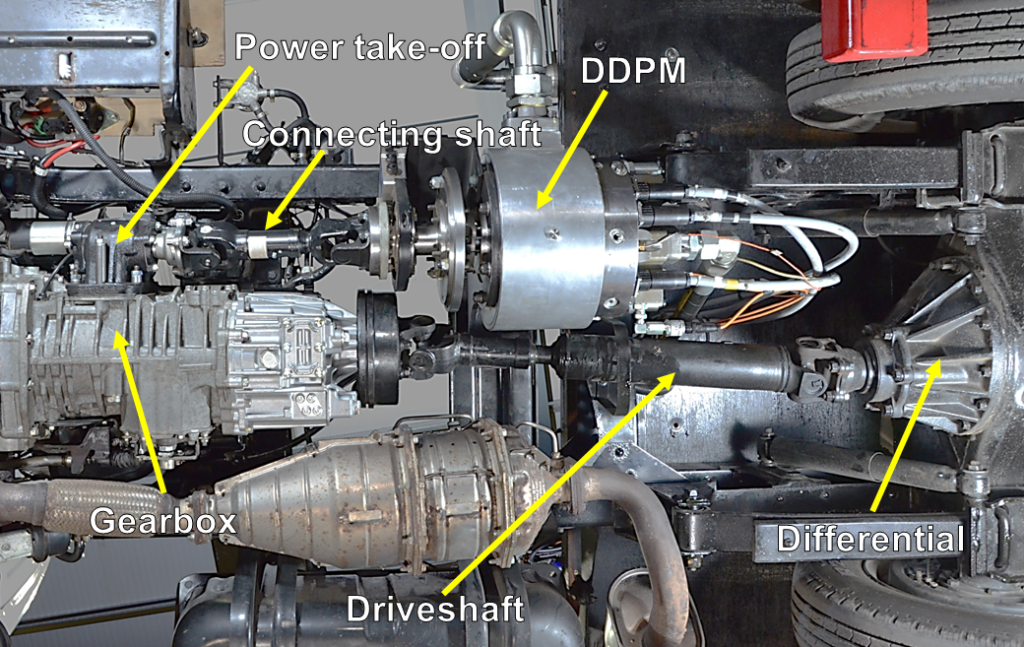
Danfoss converted a light truck to a hydraulic hybrid using a Digital Displacement® pump/motor. (A pump/motor can produce negative [braking] torque and a positive [accelerating] torque, rather than just one or the other.) The system stores recovered energy in a high-pressure hydraulic accumulator.
The underside of the converted vehicle.
Test Results
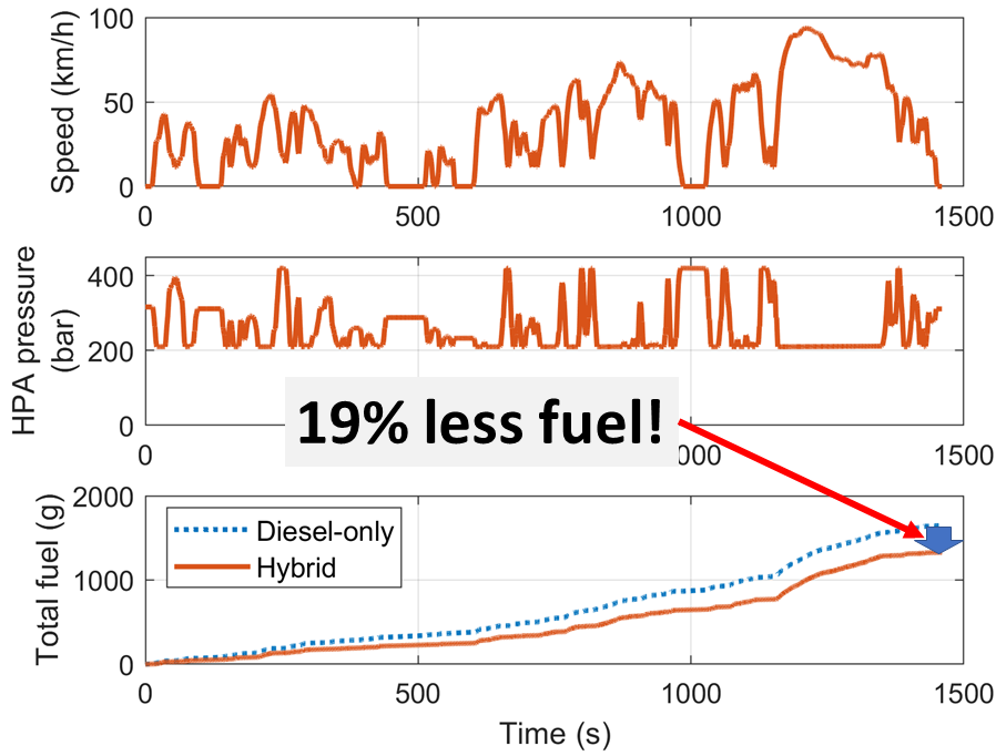
First, we checked to see how consistent the drivers were. They were remarkably consistent; the distance covered in the tests had a standard deviation of 0.3%! After that, we checked the results from the logging equipment to make sure it was sensible.
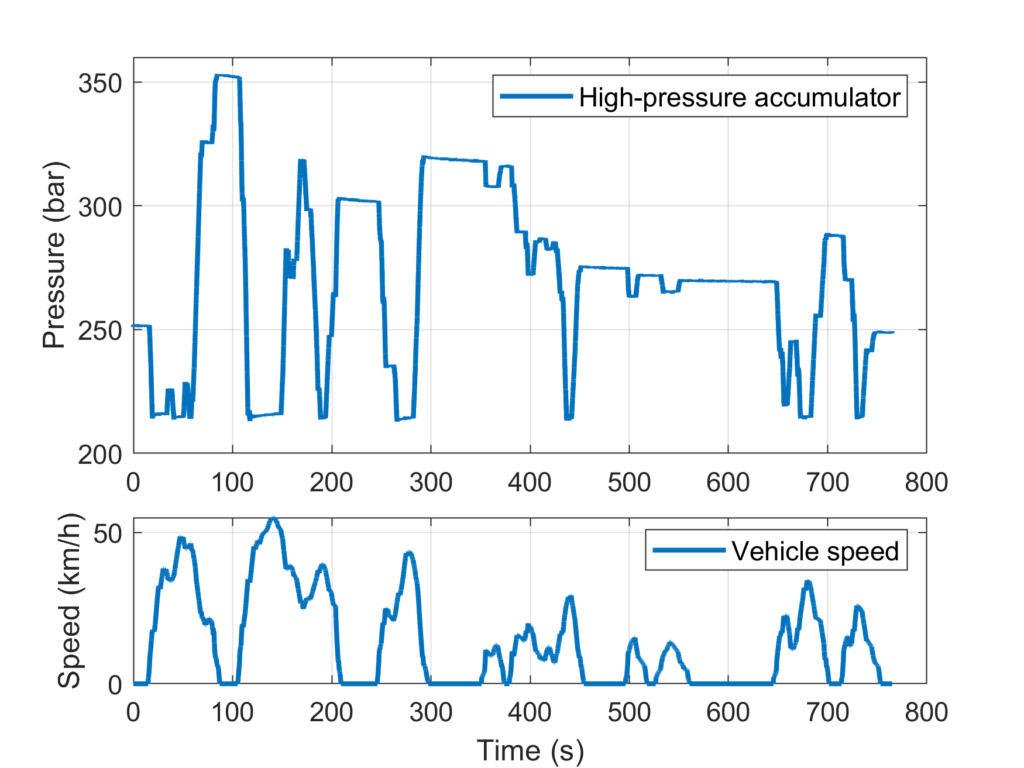
Test results showing how the pressure in the high-pressure accumulator varies with speed. Looking good!
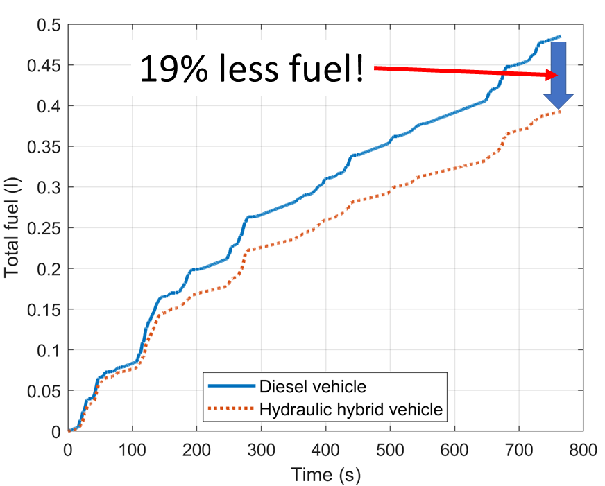
Next, we looked at how the fuel usage of the hybrid vehicle compared to the un-altered vehicle. (Hint: it used a lot less fuel!)
In testing, the hydraulic hybrid truck used 19% less fuel!
Model Validation
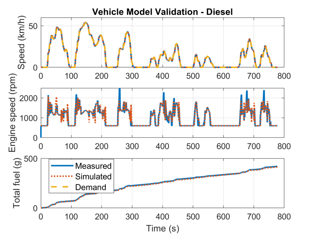
After that, we checked to make sure our model was a reasonable fit with the experimental data .(This step is called ‘validation‘, and is a common technique in engineering.)
Making sure the model and the test data match. Looking good!
Model Performance
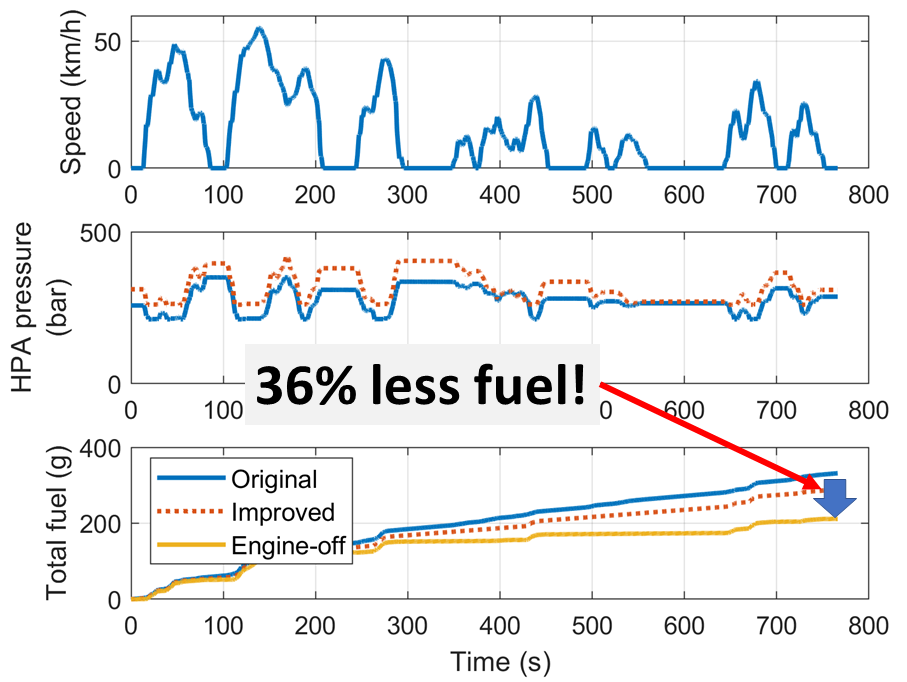
Now that we had a working model, the next step was to use this model to investigate what benefits might be achievable if we could change some of the system parameters. We found that with some small parameter changes, and by turning off the engine when it wasn’t being used, the vehicle would use much less fuel. It used 36% less fuel over this cycle!
Our modelling showed that the hybrid truck used 36% less fuel over the JE05 driving cycle!
Next, we looked at the performance on a more common drive cycle, the WLTP cycle. In this case the hybrid truck used 19% less fuel than the original diesel vehicle – not bad!
Modelling results showing that the hybrid truck uses 19% less fuel over the WLTP drive cycle.
Conclusions
The main conclusions of our paper were:
It’s possible to use Digital Displacement technology to make a hydraulic hybrid truck.
Hybridising the vehicle reduces fuel consumption by 19-36%, depending on the drive cycle.
If you want more information, please check out the full paper online.
We made a detailed model of a bi-mode rail vehicle and used control to reduce its carbon emissions (decarbonisation).
The Rail Vehicle Model
A bi-mode train is one that can run on electricity from overhead wires (sometimes called overhead line equipment or OLE), or by generating electricity from the on-board diesel generator. Then we used vehicle data to make sure the model represented the behaviour of the real train.
Control for Decarbonisation
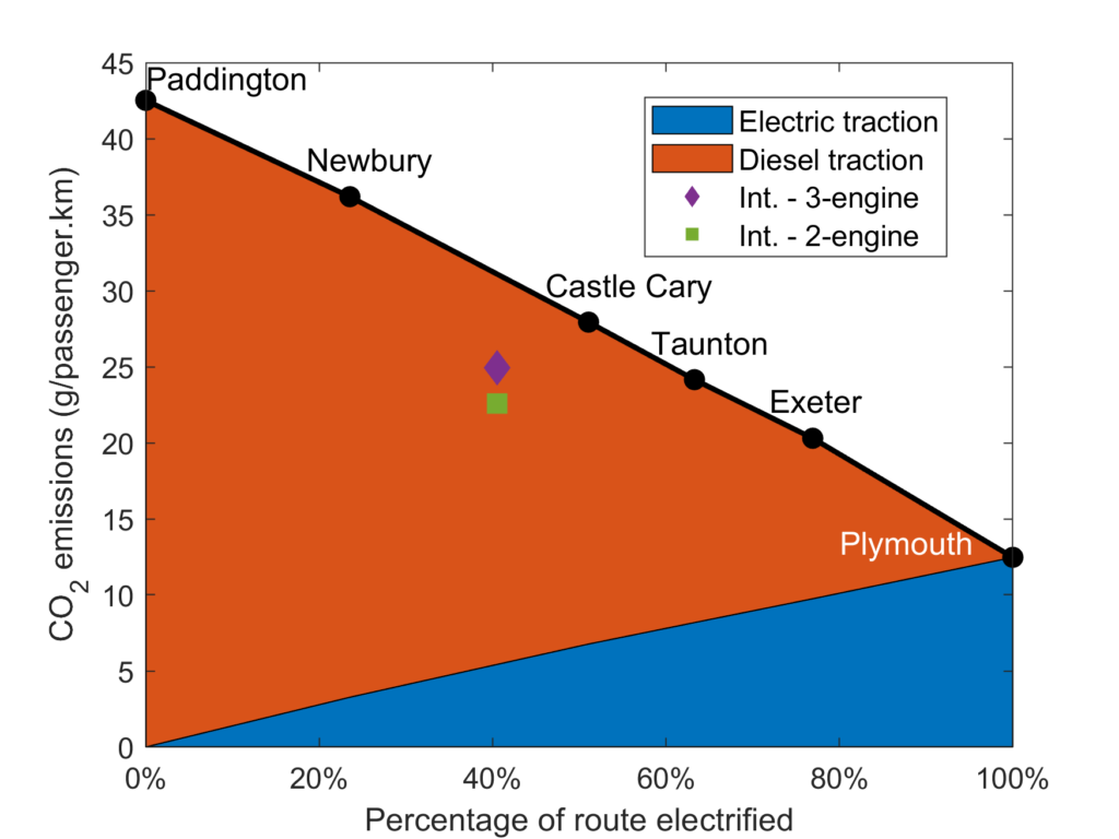
We used that model to look at a range of controllers for reducing the CO2 emitted by the train (decarbonisation) during its run from London Paddington to Plymouth in the UK. Our controller reduced the CO2 emissions of the train by 19%. Without this controller, the train produces around 42g of CO2 per passenger-kilometre of diesel running.
Intermittent Electrification
We also investigated some simple ‘intermittent electrification’, where only some sections the route are electrified. (Some people also call this discontinuous or discrete electrification.) You can see the results of this analysis in the picture, below.
This figure shows the key conclusions of the paper. Firstly, that electrification will reduce the CO2 emissions of the route (but not to zero, because the UK still produces electricity using some fossil fuels). Secondly, that intermittent electrification (only electrifying some pieces of track) and using selective engine shutdown can reduce the CO2 emissions when only part of the track is electrified.
The figure shows that intermittent electrification can be more effective than continuous electrification at reducing carbon dioxide emissions. It also shows that selective engine shutdown can be used for the decarbonisation of a bi-mode rail vehicle.
If you’d like more information on my work on railway decarbonisation, check out the project webpage, or get in touch!
We use cookies on our website to give you the most relevant experience by remembering your preferences and repeat visits. By clicking “Accept All”, you consent to the use of ALL the cookies. However, you may visit "Cookie Settings" to provide a controlled consent.
This website uses cookies to improve your experience while you navigate through the website. Out of these, the cookies that are categorized as necessary are stored on your browser as they are essential for the working of basic functionalities of the website. We also use third-party cookies that help us analyze and understand how you use this website. These cookies will be stored in your browser only with your consent. You also have the option to opt-out of these cookies. But opting out of some of these cookies may affect your browsing experience.
Necessary cookies are absolutely essential for the website to function properly. These cookies ensure basic functionalities and security features of the website, anonymously.
Cookie
Duration
Description
cookielawinfo-checkbox-analytics
11 months
This cookie is set by GDPR Cookie Consent plugin. The cookie is used to store the user consent for the cookies in the category "Analytics".
cookielawinfo-checkbox-functional
11 months
The cookie is set by GDPR cookie consent to record the user consent for the cookies in the category "Functional".
cookielawinfo-checkbox-necessary
11 months
This cookie is set by GDPR Cookie Consent plugin. The cookies is used to store the user consent for the cookies in the category "Necessary".
cookielawinfo-checkbox-others
11 months
This cookie is set by GDPR Cookie Consent plugin. The cookie is used to store the user consent for the cookies in the category "Other.
cookielawinfo-checkbox-performance
11 months
This cookie is set by GDPR Cookie Consent plugin. The cookie is used to store the user consent for the cookies in the category "Performance".
viewed_cookie_policy
11 months
The cookie is set by the GDPR Cookie Consent plugin and is used to store whether or not user has consented to the use of cookies. It does not store any personal data.
Functional cookies help to perform certain functionalities like sharing the content of the website on social media platforms, collect feedbacks, and other third-party features.
Performance cookies are used to understand and analyze the key performance indexes of the website which helps in delivering a better user experience for the visitors.
Analytical cookies are used to understand how visitors interact with the website. These cookies help provide information on metrics the number of visitors, bounce rate, traffic source, etc.
Advertisement cookies are used to provide visitors with relevant ads and marketing campaigns. These cookies track visitors across websites and collect information to provide customized ads.